User guide

Level 0 to Level 3 processing

Two components are needed to perform Level 0 to Level 3 processing: - A Level 0 dataset file (.txt), or a collection of Level 0 dataset files - A station config file (.toml)

Two test station datasets and config files are available with pypromice as an example of the Level 0 to Level 3 processing. These can be found on the Github repo here, in the src/pypromice/test/ directory in the cloned repo.

These can be processed from Level 0 to a Level 3 data product as an AWS object in pypromice.

from pypromice.process import AWS

# Define input paths
config = "src/pypromice/test/test_config1.toml"
inpath = "src/pypromice/test/"

# Initiate and process
a = AWS(config, inpath)
a.process()

# Get Level 3
l3 = a.L3

All processing steps are executed in AWS.process. These can also be broken down into each Level processing

from pypromice.process import AWS

# Define input paths
config = "src/pypromice/test/test_config2.toml"
inpath = "src/pypromice/test/"

# Initiate
a = AWS(config, inpath)

# Process to Level 1
a.getL1()
l1 = a.L1

# Process to Level 2
a.getL2()
l2 = a.L2

# Process to Level 3
a.getL3()
l3 = a.L3

Level 3 data can be saved as both NetCDF and csv formatted files using the AWS.write function.

a.write("src/pypromice/test/")

The Level 0 to Level 3 processing can also be executed from a CLI using the getL3 command.

$ get_l3 -c src/pypromice/test/test_config1.toml -i src/pypromice/test -o src/pypromice/test

Loading our data

Import from Dataverse (no downloads!)

The automated weather station (AWS) datasets from the PROMICE and GC-Net monitoring programmes are openly available on the GEUS Dataverse. These can be imported directly with pypromice, with no downloading required.

import pypromice.get as pget

# Import AWS data from station KPC_U
df = pget.aws_data("kpc_u_hour.csv")

All available AWS datasets are retrieved by station name. Use aws_names() to list all station names which can be used as an input to aws_data().

n = pget.aws_names()
print(n)

Download with pypromice

AWS data can be downloaded to file with pypromice. Open up a CLI and use the getData command.

$ get_promice_data -n KPC_U_hour.csv

Files are downloaded to the current directory as a CSV formatted file. Use the -h help flag to explore further input variables.

$ get_promice_data -h

Note

Currently, this functionality within pypromice is only for our hourly AWS data. For daily and monthly AWS data, please download these from the GEUS Dataverse.

Load from NetCDF file

AWS data can be loaded from a local NetCDF file with xarray.

import xarray as xr
ds = xr.open_dataset("KPC_U_hour.nc")

Load from CSV file

AWS data can be loaded from a local CSV file and handled as a pandas.DataFrame.

import pandas as pd
df = pd.read_csv("KPC_U_hour.csv", index_col=0, parse_dates=True)

If you would rather handle the AWS data as an xarray.Dataset object then the pandas.DataFrame can be converted.

ds = xr.Dataset.from_dataframe(df)

Plotting our data

Once loaded, variables from an AWS dataset can be simply plotted with using pandas or xarray.

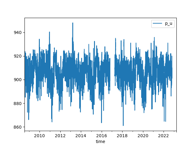
# Plot variable with pandas
# In this case, we will plot air pressure
df.plot(kind='line', y='p_u', use_index=True)

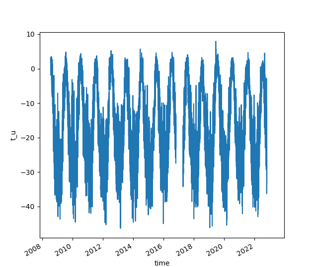
https://raw.githubusercontent.com/GEUS-Glaciology-and-Climate/geus-glaciology-and-climate.github.io/master/assets/images/kpc_u_pandas_plot.png

# Plot variable with xarray
# In this case, we will plot air temperature
ds['t_u'].plot()

https://raw.githubusercontent.com/GEUS-Glaciology-and-Climate/geus-glaciology-and-climate.github.io/master/assets/images/kpc_u_xr_plot.png

Note

Variable names are provided in the dataset metadata, or can be found on in our variables look-up table. For more complex plotting, please see either the xarray or pandas plotting documentation.

Warning

Plotting with either xarray or pandas requires matplotlib. This is not supplied as a dependency with pypromice, so please install matplotlib separately if you wish to do so.